 S'abonner à un flux RSS
Utilisateur:Jean-Michel Tanguy/SujetENTPE2023/Emeline/Jallet : Différence entre versions
| Ligne 68 : | Ligne 68 : | ||
Avec pour conditions aux limites : | Avec pour conditions aux limites : | ||
| − | <math> \phi_0^0=1 </math> et | + | ::<math> \phi_0^0=1 </math> et |
| − | <math> \phi_{0, x}^L={ik}\phi_0^L </math> | + | ::<math> \phi_{0, x}^L={ik}\phi_0^L </math> |
on a <math> B=1</math> et <math>A=\frac{ik}{(1-ikL)}</math> | on a <math> B=1</math> et <math>A=\frac{ik}{(1-ikL)}</math> | ||
Détail pour trouver A: | Détail pour trouver A: | ||
| − | <math> \phi_{0, x}^L={ik}\phi_0^L </math> | + | :<math> \phi_{0, x}^L={ik}\phi_0^L </math> |
| − | <math> \iff A=\frac{ik}{(AL+1)}</math> | + | :<math> \iff A=\frac{ik}{(AL+1)}</math> |
| − | <math> \iff A=\frac{ik}{(1-ikL)}</math> | + | :<math> \iff A=\frac{ik}{(1-ikL)}</math> |
| − | Ainsi <math> \phi_0(x)=(\frac{ik}{(1-ikL)})x+1</math> | + | :Ainsi <math> \phi_0(x)=(\frac{ik}{(1-ikL)})x+1</math> |
| Ligne 83 : | Ligne 83 : | ||
Puis à l'ordre 1: | Puis à l'ordre 1: | ||
| − | <math> \phi_{1,xx}(x)={-k^2}\phi_0(x) </math> | + | ::<math> \phi_{1,xx}(x)={-k^2}\phi_0(x) </math> |
donc par double intégration on a : | donc par double intégration on a : | ||
| − | <math> \phi_1(x) = -k^2\int\phi_0dxdx +Ax+B</math>. | + | ::<math> \phi_1(x) = -k^2\int\phi_0dxdx +Ax+B</math>. |
Avec pour conditions aux limites : | Avec pour conditions aux limites : | ||
| − | <math> \phi_1^0=0 </math> | + | ::<math> \phi_1^0=0 </math> |
et | et | ||
| − | <math> \phi_{1, x}^L={ik}\phi_1^L </math> | + | ::<math> \phi_{1, x}^L={ik}\phi_1^L </math> |
| − | on a <math> B=0 </math> | + | on a |
| − | et <math> A=\frac{-k^2L(k^2L^2+3ikL-3)}{3(1-ikL)^2}</math> | + | ::<math> B=0 </math> |
| + | et | ||
| + | ::<math> A=\frac{-k^2L(k^2L^2+3ikL-3)}{3(1-ikL)^2}</math> | ||
Calcul de A : | Calcul de A : | ||
| − | <math> \phi_1(x)= -k^2(({ik}/({1-ikL})6)x^3+x^2/2+Ax</math> | + | ::<math> \phi_1(x)= -k^2(({ik}/({1-ikL})6)x^3+x^2/2+Ax</math> |
en x=L: | en x=L: | ||
| − | <math> \phi_{1, x}^L={ik}\phi_1^L </math> | + | ::<math> \phi_{1, x}^L={ik}\phi_1^L </math> |
| − | <math> \iff \frac{ikL^2}{(1-ikL)^2}+L+A=\frac{ik(ikL^3)}{(1-ikL)*6}+\frac{L^2}{2}+AL</math> | + | ::<math> \iff \frac{ikL^2}{(1-ikL)^2}+L+A=\frac{ik(ikL^3)}{(1-ikL)*6}+\frac{L^2}{2}+AL</math> |
en isolant A dans l'équation on retrouve : | en isolant A dans l'équation on retrouve : | ||
| − | <math> A=\frac{-k^2L(k^2L^2+3ikL-3)}{3(1-ikL)^2}</math> | + | ::<math> A=\frac{-k^2L(k^2L^2+3ikL-3)}{3(1-ikL)^2}</math> |
On a donc : | On a donc : | ||
| − | <math> \phi_{1}(x)= -\frac{k^2L(k^2L^2+3ikL-3)}{3(1-ikL)^2}x-k^2(\frac{ik}{6(1-ikL)})x^3+\frac{x^2}{2}</math> | + | ::<math> \phi_{1}(x)= -\frac{k^2L(k^2L^2+3ikL-3)}{3(1-ikL)^2}x-k^2(\frac{ik}{6(1-ikL)})x^3+\frac{x^2}{2}</math> |
| Ligne 121 : | Ligne 123 : | ||
A partir des valeurs numériques suivantes : | A partir des valeurs numériques suivantes : | ||
| − | <math>k=\frac{1}{100}</math> (nombre d'onde en m<sup>-1</sup>) | + | ::<math>k=\frac{1}{100}</math> (nombre d'onde en m<sup>-1</sup>) |
| − | <math>H=40</math> (profondeur en m) | + | ::<math>H=40</math> (profondeur en m) |
| − | <math>c=\sqrt{gH}</math> (célérité de l'onde en m/s) | + | ::<math>c=\sqrt{gH}</math> (célérité de l'onde en m/s) |
| − | <math>\lambda=\frac{2\pi}{k}</math> (longueur d'onde en m) | + | ::<math>\lambda=\frac{2\pi}{k}</math> (longueur d'onde en m) |
| − | <math>L=2\lambda</math> (longueur du domaine en m) | + | ::<math>L=2\lambda</math> (longueur du domaine en m) |
[[File:Gif cas 1.gif | 400px]] | [[File:Gif cas 1.gif | 400px]] | ||
| Ligne 136 : | Ligne 138 : | ||
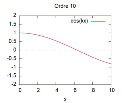
On regarde la convergence de la méthode par homotopie en fonction du produit kL. | On regarde la convergence de la méthode par homotopie en fonction du produit kL. | ||
| − | Cas kL=0,25 [[File: cas 1 ordre 10 kL = 0,25.png|400px]] | + | :Cas kL=0,25 [[File: cas 1 ordre 10 kL = 0,25.png|400px]] |
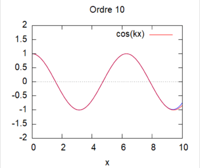
| − | Cas kL=1 [[File:cas 1 ordre 10 kL = 1.png|400px]] | + | :Cas kL=1 [[File:cas 1 ordre 10 kL = 1.png|400px]] |
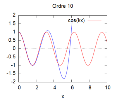
| − | Cas kL=2 [[File:cas 1 ordre 10 kL = 2.png|400px]] | + | :Cas kL=2 [[File:cas 1 ordre 10 kL = 2.png|400px]] |
=== '''Cas N°2''' === | === '''Cas N°2''' === | ||
| Ligne 148 : | Ligne 150 : | ||
==== Méthode analytique ==== | ==== Méthode analytique ==== | ||
| − | Comme pour le cas N°1, l'équation de Berkhoff à une dimension s'écrit <math> \phi_{xx} + k^2\phi = 0 </math> | + | :Comme pour le cas N°1, l'équation de Berkhoff à une dimension s'écrit <math> \phi_{xx} + k^2\phi = 0 </math> |
Ce qui nous donne comme forme pour <math> \phi </math> : <math> \phi(x) = Ae^{ikx} + Be^{-ikx} </math> | Ce qui nous donne comme forme pour <math> \phi </math> : <math> \phi(x) = Ae^{ikx} + Be^{-ikx} </math> | ||
| Ligne 154 : | Ligne 156 : | ||
On peut déterminer les constantes A et B avec les conditions initiales de ce cas. | On peut déterminer les constantes A et B avec les conditions initiales de ce cas. | ||
| − | <math> \phi_{x}(0) = ik(2 - \phi(0)) \iff ik(A - B) = ik(2 - A - B) </math> | + | ::<math> \phi_{x}(0) = ik(2 - \phi(0)) \iff ik(A - B) = ik(2 - A - B) </math> |
| − | <math> \iff A = 1 </math> | + | ::<math> \iff A = 1 </math> |
| − | Et <math> \phi_{x}(L) = 0 \iff ik(Ae^{ikL} - Be^{-ikL}) = 0 \iff B = e^{2ikL} </math> | + | Et |
| + | ::<math> \phi_{x}(L) = 0 \iff ik(Ae^{ikL} - Be^{-ikL}) = 0 \iff B = e^{2ikL} </math> | ||
| − | Ainsi <math> \phi(x)= e^{ikx} + e^{2ikL}e^{-ikx} </math> | + | Ainsi |
| + | ::<math> \phi(x)= e^{ikx} + e^{2ikL}e^{-ikx} </math> | ||
| − | La solution réelle associée à cette fonction est <math> h(x) = cos(kx) + cos(2kL+kx) </math> | + | :La solution réelle associée à cette fonction est <math> h(x) = cos(kx) + cos(2kL+kx) </math> |
==== Méthode par homotopie ==== | ==== Méthode par homotopie ==== | ||
| − | En procédant de la même manière que dans le cas 1 on retrouve comme relation d'homotopie : | + | :En procédant de la même manière que dans le cas 1 on retrouve comme relation d'homotopie : |
| − | <math> (1- p)(\phi_{0,xx}(x)+p\phi_{1,xx}(x)+p^2\phi_{2,xx}(x)+...)+p[\phi_{0,xx}(x)+p\phi_{1,xx}(x)+p^2\phi_{2,xx}(x)+...+k^2(\phi_0(x)+p\phi_0(x)+p^2\phi_2(x)+...)]=0 </math> | + | ::<math> (1- p)(\phi_{0,xx}(x)+p\phi_{1,xx}(x)+p^2\phi_{2,xx}(x)+...)+p[\phi_{0,xx}(x)+p\phi_{1,xx}(x)+p^2\phi_{2,xx}(x)+...+k^2(\phi_0(x)+p\phi_0(x)+p^2\phi_2(x)+...)]=0 </math> |
===== Ordre 0 ===== | ===== Ordre 0 ===== | ||
| Ligne 173 : | Ligne 177 : | ||
Tout d'abord, à l'ordre 0: | Tout d'abord, à l'ordre 0: | ||
| − | <math> \phi_{0,xx}(x)=0 </math> | + | ::<math> \phi_{0,xx}(x)=0 </math> |
Par intégration on a : | Par intégration on a : | ||
| − | <math> \phi_0(x)=Ax+B </math> | + | ::<math> \phi_0(x)=Ax+B </math> |
Avec les conditions aux limites : | Avec les conditions aux limites : | ||
| − | <math> \phi_{0,x}^0=ik(2-\phi) </math> et | + | ::<math> \phi_{0,x}^0=ik(2-\phi) </math> et |
<math> \phi_{0, x}^L=0 </math> | <math> \phi_{0, x}^L=0 </math> | ||
On a : | On a : | ||
| − | <math> A = 0 </math> et | + | ::<math> A = 0 </math> |
| − | <math> B = 2 </math> | + | et |
| + | ::<math> B = 2 </math> | ||
| − | Donc <math> \phi_0(x)=2 </math> | + | Donc |
| + | ::<math> \phi_0(x)=2 </math> | ||
===== Ordre 1 ===== | ===== Ordre 1 ===== | ||
| Ligne 194 : | Ligne 200 : | ||
Ensuite, pour l'ordre 1: | Ensuite, pour l'ordre 1: | ||
| − | On a <math> \phi_{1,xx}(x) = -k^{2}\phi_0(x) </math> | + | On a |
| + | ::<math> \phi_{1,xx}(x) = -k^{2}\phi_0(x) </math> | ||
| − | donc <math> \phi_1 (x) = -k^2x^2 + Ax + B </math> | + | donc |
| + | ::<math> \phi_1 (x) = -k^2x^2 + Ax + B </math> | ||
Avec les conditions initiales on trouve pour A et B : | Avec les conditions initiales on trouve pour A et B : | ||
| − | <math> A = 2k^2L </math> et <math> B = 2ikL </math> | + | ::<math> A = 2k^2L </math> et <math> B = 2ikL </math> |
| − | Donc <math> \phi_1 (x) = - k^2x^2 + 2k^2Lx + 2ikL </math> | + | Donc |
| + | ::<math> \phi_1 (x) = - k^2x^2 + 2k^2Lx + 2ikL </math> | ||
[[File:Gif cas 2 Thomas et Emeline.gif|400px]] | [[File:Gif cas 2 Thomas et Emeline.gif|400px]] | ||
| Ligne 210 : | Ligne 219 : | ||
=== '''Cas N°3''' === | === '''Cas N°3''' === | ||
| − | Dans ce cas, nous nous placerons dans un domaine monodimensionnel plat de longueur L avec une pente de fond constante (s=cst). L'entrée se fait par l'aval avec une onde de fréquence unitaire <math> \phi_{x} =ik(2−\phi) </math> et la sortie en amont <math> \phi_{x}(x=L)=ik\phi(x=L) </math>. | + | :Dans ce cas, nous nous placerons dans un domaine monodimensionnel plat de longueur L avec une pente de fond constante (s=cst). L'entrée se fait par l'aval avec une onde de fréquence unitaire <math> \phi_{x} =ik(2−\phi) </math> et la sortie en amont <math> \phi_{x}(x=L)=ik\phi(x=L) </math>. |
==== Résolution analytique ==== | ==== Résolution analytique ==== | ||
| − | Le problème est complexifié puisque H(x) n'est plus égal à <math>H_0</math> mais à <math>H_0-sx</math>. | + | :Le problème est complexifié puisque H(x) n'est plus égal à <math>H_0</math> mais à <math>H_0-sx</math>. |
| − | On a toujours <math> \nabla.(CC_g\nabla \phi)+k^2CC_g\phi=0 </math> mais avec <math> C=C_g=\sqrt{gH(x)} </math> | + | :On a toujours <math> \nabla.(CC_g\nabla \phi)+k^2CC_g\phi=0 </math> mais avec <math> C=C_g=\sqrt{gH(x)} </math> |
| − | Soit <math>{\displaystyle H(x)\frac{\partial^2 \phi}{\partial x^2} -\frac{\partial \phi}{\partial x} + k^2H(x) \phi = 0} </math> | + | Soit |
| + | ::<math>{\displaystyle H(x)\frac{\partial^2 \phi}{\partial x^2} -\frac{\partial \phi}{\partial x} + k^2H(x) \phi = 0} </math> | ||
| − | Nous utilisons le changement de variable : <math> z=H_0-sx</math>. | + | :Nous utilisons le changement de variable : <math> z=H_0-sx</math>. |
| − | Et nous prenons: <math> s = \frac{1/200} \ </math>. | + | :Et nous prenons: <math> s = \frac{1/200} \ </math>. |
| − | Nous nous intéressons au cas <math> k=ko\sqrt{Ho/H(x)} </math>. | + | :Nous nous intéressons au cas <math> k=ko\sqrt{Ho/H(x)} </math>. |
Soit l'équation à résoudre : | Soit l'équation à résoudre : | ||
| − | <math> (H_0-sx)\phi_{xx}-s\phi_{x}+k^2(H_0-sx)\phi=0 </math> | + | ::<math> (H_0-sx)\phi_{xx}-s\phi_{x}+k^2(H_0-sx)\phi=0 </math> |
On cherche une solution de la forme de l'équation de Bessel, c'est à dire de la forme : <math> z^2\phi_{zz}+z\phi_{z}+(\dfrac{k^2}{s^2})z^2\phi=0 </math> | On cherche une solution de la forme de l'équation de Bessel, c'est à dire de la forme : <math> z^2\phi_{zz}+z\phi_{z}+(\dfrac{k^2}{s^2})z^2\phi=0 </math> | ||
| − | <math>\phi(z)=AJ_0(\dfrac{k}{s}z)+BY_0(\dfrac{k}{s}z)</math> | + | ::<math>\phi(z)=AJ_0(\dfrac{k}{s}z)+BY_0(\dfrac{k}{s}z)</math> |
Avec les conditions limites : | Avec les conditions limites : | ||
| − | <math>\phi(x=0)=1</math> | + | ::<math>\phi(x=0)=1</math> et <math>\phi_x(x=L)=ik \phi(x=L) </math> |
| − | et | + | |
| − | <math>\phi_x(x=L)=ik \phi(x=L) </math> | + | |
Ce qui donne avec le changement de variable : | Ce qui donne avec le changement de variable : | ||
| − | <math>\phi(z=H_0)=1</math> | + | ::<math>\phi(z=H_0)=1</math> |
| − | et <math>\phi_z(z=H_0-sL)=ik \phi(z=H_0-sL) </math> | + | et |
| + | ::<math>\phi_z(z=H_0-sL)=ik \phi(z=H_0-sL) </math> | ||
| Ligne 247 : | Ligne 256 : | ||
| − | <math> {\phi(z)=\frac{iY_0^L - Y_1^L}{J_0^0(iY_0^L - Y_1^L) + Y_0^0 (J_1^L-i J_0^L)} J_0 (2 \alpha \sqrt{z}) + \frac{J_1^L - i J_0^L}{J_0^0 (i Y_0^L-Y_1^L) + Y_0^0 (J_1^L - i J_0^L)} Y_0 (2 \alpha \sqrt{z})} </math> | + | ::<math> {\phi(z)=\frac{iY_0^L - Y_1^L}{J_0^0(iY_0^L - Y_1^L) + Y_0^0 (J_1^L-i J_0^L)} J_0 (2 \alpha \sqrt{z}) + \frac{J_1^L - i J_0^L}{J_0^0 (i Y_0^L-Y_1^L) + Y_0^0 (J_1^L - i J_0^L)} Y_0 (2 \alpha \sqrt{z})} </math> |
==== Résolution par homotopie ==== | ==== Résolution par homotopie ==== | ||
| − | Soit la relation d'homotopie suivante : <math>(1-p)\phi_{xx}+p(H_0-sx)\phi_{xx}-s\phi_{x}+k^2(H_0-sx)\phi=0</math> | + | :Soit la relation d'homotopie suivante : <math>(1-p)\phi_{xx}+p(H_0-sx)\phi_{xx}-s\phi_{x}+k^2(H_0-sx)\phi=0</math> |
| − | ordre 0 | + | ===== ordre 0 ===== |
| − | <math>\phi_{xx}=0</math> donc on a <math>\phi_0=Ax+B</math> | + | ::<math>\phi_{xx}=0</math> donc on a <math>\phi_0=Ax+B</math> |
et avec les conditions initiales on trouve : | et avec les conditions initiales on trouve : | ||
| − | <math>\phi_0=\frac{ik}{1-ikL}x+1</math> | + | ::<math>\phi_0=\frac{ik}{1-ikL}x+1</math> |
La simulation sur WXMaxima nous donne pour le produit kL=1 le gif suivant : | La simulation sur WXMaxima nous donne pour le produit kL=1 le gif suivant : | ||
| Ligne 269 : | Ligne 278 : | ||
Dans ce cas nous avons une vague sphérique générée par une source sinusoïdale | Dans ce cas nous avons une vague sphérique générée par une source sinusoïdale | ||
| − | <math> | + | ::<math> |
\begin{cases} \Delta \phi + k^2\phi=0, \\ \phi^{r=r_0}=1, \\\phi_r^{r=R}=ik\phi^{r=R}. \end{cases} | \begin{cases} \Delta \phi + k^2\phi=0, \\ \phi^{r=r_0}=1, \\\phi_r^{r=R}=ik\phi^{r=R}. \end{cases} | ||
</math> | </math> | ||
Et en coordonnées polaires : | Et en coordonnées polaires : | ||
| − | <math> | + | ::<math> |
\begin{cases} \phi_{rr}+\dfrac{1}{r}\phi_r + k^2\phi=0, \\ \phi^{r=r_0}=1, \\\phi_r^{r=R}=ik\phi^{r=R}. \end{cases} | \begin{cases} \phi_{rr}+\dfrac{1}{r}\phi_r + k^2\phi=0, \\ \phi^{r=r_0}=1, \\\phi_r^{r=R}=ik\phi^{r=R}. \end{cases} | ||
</math> | </math> | ||
| − | avec <math> r_0=1m </math>, <math> R=100m </math> et <math> k=0.1m^{-1} </math>. | + | :avec <math> r_0=1m </math>, <math> R=100m </math> et <math> k=0.1m^{-1} </math>. |
Version du 6 juin 2023 à 17:45
Sommaire |
Modèle de Berkhoff
- La houle peut être modélisée par l'équation aux dérivées partielles (EDP) issue du modèle de Berkhoff suivante :
- $ \nabla.(CC_g\nabla \phi)+k^2CC_g\phi=0 $
- Avec :
$ \phi $ : le potentiel, k : le nombre d’onde, fonction de la profondeur H et de la fréquence $ \omega $, C : la célérité de l’onde, Cg : la célérité de groupe des vagues.
Résolution
- Pour résoudre cette équation, nous utiliserons une méthode analytique lorsque cela sera possible et une méthode par homotopie.
- Nous nous placerons dans différent cas pour résoudre cette équation.
Cas N°1
- Pour ce premier cas, nous étudierons le cas d'un canal monodimensionnel plat de longueur L avec entrée par l'aval d'une onde de fréquence unitaire $ \phi=1 $(condition de Dirichlet) et sortie libre amont $ \phi_{x}=ik\phi $ (condition de Robin).
Méthode analytique
- Dans cette situation l'équation issue du modèle de Berkhoff s'écrit : $ \phi_{xx} + k^2\phi=0 $.
Soit $ \phi(x) = Ae^{ikx}+Be^{-ikx} $ , A et B sont des constantes à déterminer avec les conditions initiales.
- En aval pour x=0, $ \phi=1 $
donc $ A + B = 1 $
- En amont pour x = L, $ \phi_{x}(L)=ik\phi{L} $
Donc $ ikAe^{ikL} - ikBe^{-ikL} = ik(Ae^{ikL} + Be^{-ikL}) $.
- Ainsi A = 1 et B = 0
La solution analytique de cette équation est donc $ \phi(x)=e^{ikx} $
On s'intéresse à la partie réelle de $ \phi e^{i\omega t} $. Ainsi $ h(x,t) = cos(kx+ \omega t) $
Méthode par homotopie
- En choisissant la dérivée seconde comme fonction auxiliaire linéaire et en partant d'une solution initiale nulle, la relation d'homotopie devient :
- $ (1-p)\phi_{xx}+ p(\phi_{xx}+k^2\phi)=0 $
Or
- $ \phi(x,p)=\phi_0(x)+p\phi_1(x)+p^2\phi_2(x)+... $
Et
- $ \phi_{xx}=\phi_{0,xx}(x)+p\phi_{1,xx}(x)+p^2\phi_{2,xx}(x)+... $
Donc en injectant ces deux expressions dans la relation d'homotopie on a :
- $ (1- p)(\phi_{0,xx}(x)+p\phi_{1,xx}(x)+p^2\phi_{2,xx}(x)+...)+p[\phi_{0,xx}(x)+p\phi_{1,xx}(x)+p^2\phi_{2,xx}(x)+...+k^2(\phi_0(x)+p\phi_0(x)+p^2\phi_2(x)+...)]=0 $
Ordre 0
A l'ordre 0, on a:
- $ \phi_{xx}=0 $
donc
- $ \phi_{0,xx}(x)=0 $
En intégrant deux fois on a :
- $ \phi_0(x)=Ax+B $
Avec pour conditions aux limites :
- $ \phi_0^0=1 $ et
- $ \phi_{0, x}^L={ik}\phi_0^L $
on a $ B=1 $ et $ A=\frac{ik}{(1-ikL)} $
Détail pour trouver A:
- $ \phi_{0, x}^L={ik}\phi_0^L $
- $ \iff A=\frac{ik}{(AL+1)} $
- $ \iff A=\frac{ik}{(1-ikL)} $
- Ainsi $ \phi_0(x)=(\frac{ik}{(1-ikL)})x+1 $
Ordre 1
Puis à l'ordre 1:
- $ \phi_{1,xx}(x)={-k^2}\phi_0(x) $
donc par double intégration on a :
- $ \phi_1(x) = -k^2\int\phi_0dxdx +Ax+B $.
Avec pour conditions aux limites :
- $ \phi_1^0=0 $
et
- $ \phi_{1, x}^L={ik}\phi_1^L $
on a
- $ B=0 $
et
- $ A=\frac{-k^2L(k^2L^2+3ikL-3)}{3(1-ikL)^2} $
Calcul de A :
- $ \phi_1(x)= -k^2(({ik}/({1-ikL})6)x^3+x^2/2+Ax $
en x=L:
- $ \phi_{1, x}^L={ik}\phi_1^L $
- $ \iff \frac{ikL^2}{(1-ikL)^2}+L+A=\frac{ik(ikL^3)}{(1-ikL)*6}+\frac{L^2}{2}+AL $
en isolant A dans l'équation on retrouve :
- $ A=\frac{-k^2L(k^2L^2+3ikL-3)}{3(1-ikL)^2} $
On a donc :
- $ \phi_{1}(x)= -\frac{k^2L(k^2L^2+3ikL-3)}{3(1-ikL)^2}x-k^2(\frac{ik}{6(1-ikL)})x^3+\frac{x^2}{2} $
Ordre 2
On peut ensuite modéliser les ordres suivants grâce à WXMaxima A partir des valeurs numériques suivantes :
- $ k=\frac{1}{100} $ (nombre d'onde en m-1)
- $ H=40 $ (profondeur en m)
- $ c=\sqrt{gH} $ (célérité de l'onde en m/s)
- $ \lambda=\frac{2\pi}{k} $ (longueur d'onde en m)
- $ L=2\lambda $ (longueur du domaine en m)

Etude de sensibilité
On regarde la convergence de la méthode par homotopie en fonction du produit kL.
- Cas kL=0,25

- Cas kL=1

- Cas kL=2

Cas N°2
Dans ce cas, nous nous placerons dans un domaine monodimensionnel plat de longueur L avec entrée par l'aval d'une onde de fréquence unitaire et une condition de flux aval $ \phi_{x} =ik(2−\phi) $ et réflexion totale amont $ \phi_{x}=0 $.
Méthode analytique
- Comme pour le cas N°1, l'équation de Berkhoff à une dimension s'écrit $ \phi_{xx} + k^2\phi = 0 $
Ce qui nous donne comme forme pour $ \phi $ : $ \phi(x) = Ae^{ikx} + Be^{-ikx} $
On peut déterminer les constantes A et B avec les conditions initiales de ce cas.
- $ \phi_{x}(0) = ik(2 - \phi(0)) \iff ik(A - B) = ik(2 - A - B) $
- $ \iff A = 1 $
Et
- $ \phi_{x}(L) = 0 \iff ik(Ae^{ikL} - Be^{-ikL}) = 0 \iff B = e^{2ikL} $
Ainsi
- $ \phi(x)= e^{ikx} + e^{2ikL}e^{-ikx} $
- La solution réelle associée à cette fonction est $ h(x) = cos(kx) + cos(2kL+kx) $
Méthode par homotopie
- En procédant de la même manière que dans le cas 1 on retrouve comme relation d'homotopie :
- $ (1- p)(\phi_{0,xx}(x)+p\phi_{1,xx}(x)+p^2\phi_{2,xx}(x)+...)+p[\phi_{0,xx}(x)+p\phi_{1,xx}(x)+p^2\phi_{2,xx}(x)+...+k^2(\phi_0(x)+p\phi_0(x)+p^2\phi_2(x)+...)]=0 $
Ordre 0
Tout d'abord, à l'ordre 0:
- $ \phi_{0,xx}(x)=0 $
Par intégration on a :
- $ \phi_0(x)=Ax+B $
Avec les conditions aux limites :
- $ \phi_{0,x}^0=ik(2-\phi) $ et
$ \phi_{0, x}^L=0 $
On a :
- $ A = 0 $
et
- $ B = 2 $
Donc
- $ \phi_0(x)=2 $
Ordre 1
Ensuite, pour l'ordre 1:
On a
- $ \phi_{1,xx}(x) = -k^{2}\phi_0(x) $
donc
- $ \phi_1 (x) = -k^2x^2 + Ax + B $
Avec les conditions initiales on trouve pour A et B :
- $ A = 2k^2L $ et $ B = 2ikL $
Donc
- $ \phi_1 (x) = - k^2x^2 + 2k^2Lx + 2ikL $

Etude de sensibilité
Cas N°3
- Dans ce cas, nous nous placerons dans un domaine monodimensionnel plat de longueur L avec une pente de fond constante (s=cst). L'entrée se fait par l'aval avec une onde de fréquence unitaire $ \phi_{x} =ik(2−\phi) $ et la sortie en amont $ \phi_{x}(x=L)=ik\phi(x=L) $.
Résolution analytique
- Le problème est complexifié puisque H(x) n'est plus égal à $ H_0 $ mais à $ H_0-sx $.
- On a toujours $ \nabla.(CC_g\nabla \phi)+k^2CC_g\phi=0 $ mais avec $ C=C_g=\sqrt{gH(x)} $
Soit
- $ {\displaystyle H(x)\frac{\partial^2 \phi}{\partial x^2} -\frac{\partial \phi}{\partial x} + k^2H(x) \phi = 0} $
- Nous utilisons le changement de variable : $ z=H_0-sx $.
- Et nous prenons: $ s = \frac{1/200} \ $.
- Nous nous intéressons au cas $ k=ko\sqrt{Ho/H(x)} $.
Soit l'équation à résoudre :
- $ (H_0-sx)\phi_{xx}-s\phi_{x}+k^2(H_0-sx)\phi=0 $
On cherche une solution de la forme de l'équation de Bessel, c'est à dire de la forme : $ z^2\phi_{zz}+z\phi_{z}+(\dfrac{k^2}{s^2})z^2\phi=0 $
- $ \phi(z)=AJ_0(\dfrac{k}{s}z)+BY_0(\dfrac{k}{s}z) $
Avec les conditions limites :
- $ \phi(x=0)=1 $ et $ \phi_x(x=L)=ik \phi(x=L) $
Ce qui donne avec le changement de variable :
- $ \phi(z=H_0)=1 $
et
- $ \phi_z(z=H_0-sL)=ik \phi(z=H_0-sL) $
On obtient au final :
- $ {\phi(z)=\frac{iY_0^L - Y_1^L}{J_0^0(iY_0^L - Y_1^L) + Y_0^0 (J_1^L-i J_0^L)} J_0 (2 \alpha \sqrt{z}) + \frac{J_1^L - i J_0^L}{J_0^0 (i Y_0^L-Y_1^L) + Y_0^0 (J_1^L - i J_0^L)} Y_0 (2 \alpha \sqrt{z})} $
Résolution par homotopie
- Soit la relation d'homotopie suivante : $ (1-p)\phi_{xx}+p(H_0-sx)\phi_{xx}-s\phi_{x}+k^2(H_0-sx)\phi=0 $
ordre 0
- $ \phi_{xx}=0 $ donc on a $ \phi_0=Ax+B $
et avec les conditions initiales on trouve :
- $ \phi_0=\frac{ik}{1-ikL}x+1 $
La simulation sur WXMaxima nous donne pour le produit kL=1 le gif suivant :

Cas N°4
Dans ce cas nous avons une vague sphérique générée par une source sinusoïdale
- $ \begin{cases} \Delta \phi + k^2\phi=0, \\ \phi^{r=r_0}=1, \\\phi_r^{r=R}=ik\phi^{r=R}. \end{cases} $
Et en coordonnées polaires :
- $ \begin{cases} \phi_{rr}+\dfrac{1}{r}\phi_r + k^2\phi=0, \\ \phi^{r=r_0}=1, \\\phi_r^{r=R}=ik\phi^{r=R}. \end{cases} $
- avec $ r_0=1m $, $ R=100m $ et $ k=0.1m^{-1} $.